39 excel pivot table conditional formatting row labels
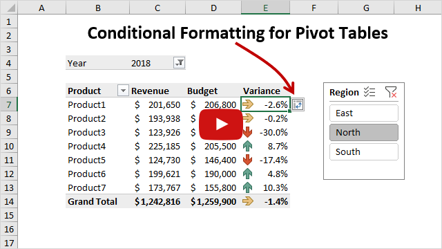
Pivot Table Conditional Formatting - Excel Pivot Tables Select a pivot table cell, and on the Ribbon's Home tab, click Conditional Formatting, then click Manage Rules. Select your pivot table rule, and click Edit Rule, to open the Edit Formatting Rule window. In the Apply Rule To section, there are 3 options, and the Selected cells option is selected. The Selected cells option works in many cases ... How to Apply Conditional Formatting to Pivot Tables - Excel Campus So in this post I explain how to apply conditional formatting for pivot tables. 1. Select a cell in the Values area The first step is to select a cell in the Values area of the pivot table. If your pivot table has multiple fields in the Values area, select a cell for the field you want to apply the formatting to. 2. Apply Conditional Formatting
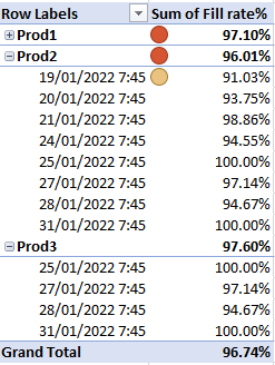
5 pivot tables you probably haven't seen before | Exceljet By setting the email count to display a percentage of row, the pivot table will show a breakdown by day of week. In addition, you add conditional formatting to make the higher and lower percentages stand out. Green for higher percentages, blue for lower percentages. Now it's clear: most sign-ups are on weekdays.
Excel pivot table conditional formatting row labels
Pivot Table Grouping, Ungrouping And Conditional Formatting 25 Oct 2022 — Conditional formatting is used to define rules to format data values in the table. It helps us to identify the important data easily in a large ... Conditional Format Pivot Table Row | Chandoo.org Excel Forums - Become ... Select the entire row, and when you apply the conditional format, make the column reference absolute. So, say we want the entire row 2 to be formatted if cell in col B = 5. formula would be: =$B2=5 Formatting Pivot Table Row Labels by Level | MrExcel Message Board hover your cursor over the top line of one of the SubTotals of the Level that you want to format until you get a downward pointing, then left click - that should highlight all the cells at that level right click while hovering over one of the selected cells to format it OR hit Ctrl+F1
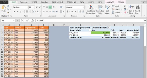
Excel pivot table conditional formatting row labels. Pivot Table Conditional Format Row Label Filter After a bit of investigation this is what I have found so far about how row filtering in a pivot table affects conditional formatting based on the format type: Format all cells based on their values - This works if you change minimum and maximum from automatic to number Format only cells that contain - Works normally Pivot Table Conditional Formatting - Computer Tutoring How to Conditionally Format an Entire Row in a Pivot Table? · First select Cell E6. · Then click Conditional Formatting - New Rule. · After that select Use a ... Conditional Formatting on Pivot Table row labels As per my knowledge, in this case it does not matter what is the source of pivot as after getting the data in pivot, it's the pivot where the conditional formatting need to be applied, please upload a sample. thanks. Regards, DILIPandey DILIPandey +91 9810929744 dilipandey@gmail.com Register To Reply How to conditional formatting pivot table in Excel? - ExtendOffice Conditional formatting pivot table 1. Select the data range you want to conditional formatting, then click Home > Conditional Formatting. Note: You only can conditional formatting the Field in Values section in the PivotTable Field List Pane. 2.
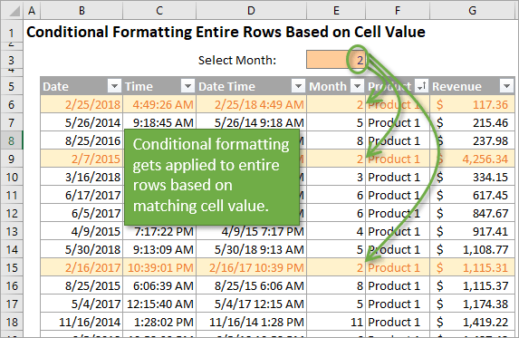
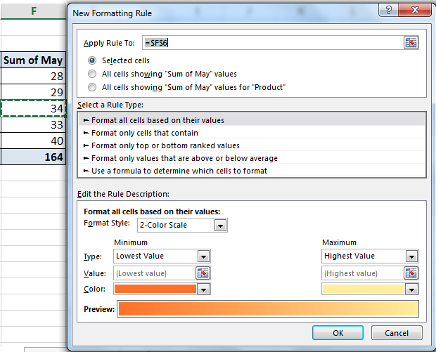
How to Apply Conditional Formatting to Rows Based on Cell Value - Excel ... On the Home tab of the Ribbon, select the Conditional Formatting drop-down and click on Manage Rules…. That will bring up the Conditional Formatting Rules Manager window. Click on New Rule. This will open the New Formatting Rule window. Under Select a Rule Type, choose Use a formula to determine which cells to format. Add Pivot Table Conditional Formatting and Fix Problems On the Ribbon's Home tab, click Conditional Formatting, then click Manage Rules In the list of rules, select the Data Bar rule, which applies to cells B3:B8 Click Edit Rule, to open the Edit Formatting Rule window. In the Apply Rule To section, select the 3rd option, All Cells Showing "Sum of Sales" Values for "YrMth" Apply Conditional Formatting | Excel Pivot Table Tutorial Go to Home Tab → Styles → Conditional Formatting → New Rule. From rule to, select the third option. And, from "select a rule" type select "Format only top or bottom" ranked values. In edit rule description, enter 1 in the input box and from the drop-down menu select "each Column Group". Apply formatting you want. Click OK. Re-Apply Pivot Table Conditional Formatting - yoursumbuddy This method relies on all the conditional formatting you want to re-apply being in that first row labels cell. In cases where the conditional formatting might not apply to the leftmost row label, I've still applied it to that column, but modified the condition to check which column it's in. This function can be modified and called from a ...
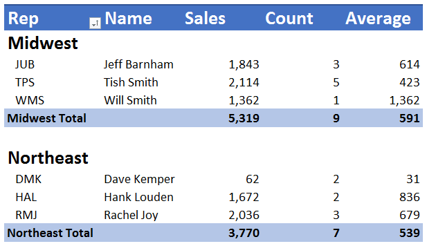
Pivot Table Conditional Formatting for Different Rows Items? May 08, 2020 · Select Your Pivot Table and: Go to Conditional Formatting -> New Rule -> Choose All cells showing "duration" values for "Type and "Date Selection" under "Apply Rule To" section -> Use a Formula to Determine which cells to format and enter the following formula: =AND(A6="Cars",A6>3), You can create new rules for other two conditions as well: Copy conditional Formatting to all rows of Pivot Table Wise people of the forum I have a little question.\. I have a pivot table that has a row of 5 columns with sales results in each. I set up a conditioning format that shows the cells in that row that exceed the average. My question is how do I copy this formatting to all the rows below without having to enter the same formula for each row. Conditional Formatting in Pivot Table - WallStreetMojo To apply conditional formatting in the pivot table, first, we must select the column to format. In this example, select "Grand Total Column." Then, in the "Home" Tab in the "Styles" section, click on "Conditional Formatting." Consequently, a dialog box pops up. Then, we need to click on "New Rule." As a result, another dialog box will pop up. Pivot Table Conditional Formatting - Microsoft Community Hub Hi all :) I have an issue conditionally formatting a Pivot Table. I have my row hierarchy set up as Region, Area, Store, Consultant. My rows are expanded out only to a Store Level. I need the Store Name to be highlighted red if the value in the first column is <1. I have applied conditional fo...
PivotTable Report Group Formatting - Excel University
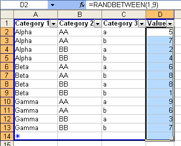
Excel VBA: Conditional Format of Pivot Table based on Column Label ... For example, if you have the following table from which you create a pivot: Product Price Cola 123 Fanta 456 Sum of Price 789 then by creating a pivot table, you will have these items: Cola, Fanta, 'Sum of Price', and the following field labels: 'Row labels', 'Sum of Price'.

How to Apply Conditional Formatting in Pivot Table? (with ...
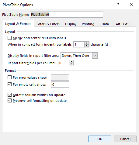
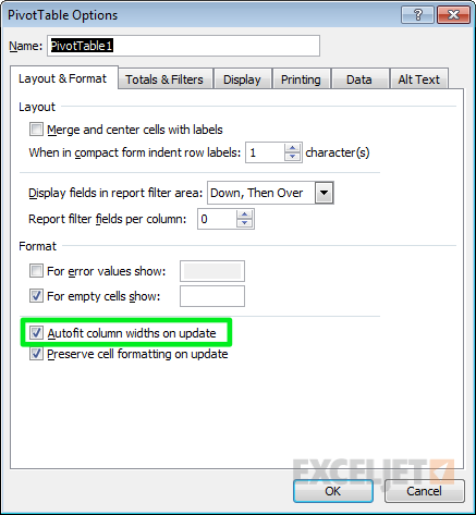
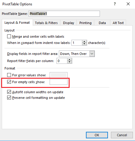
How to make row labels on same line in pivot table? - ExtendOffice Make row labels on same line with PivotTable Options You can also go to the PivotTable Options dialog box to set an option to finish this operation. 1. Click any one cell in the pivot table, and right click to choose PivotTable Options, see screenshot: 2.

Learn How to Apply Conditional Formatting in a Pivot Table ...
Pivot Table Conditional Formatting in Excel - GeeksforGeeks Basic Excel Formulas and Functions. Firstly, we can highlight the cells that are greater or less than a particular number, or are between a particular range, or are equal to a particular number. Secondly, we can highlight the cells that are the top 10 items or the bottom 10 items or occur in the top 10% or bottom 10% of that particular column ...

How to Highlight A row based on Cell Value In Pivot Table ...
How to Highlight A row based on Cell Value In Pivot Table By selecting the pivot table, the user must point to the 'Home Tab' and must click on the 'Conditional Formatting' menu. From the ' Conditional Formatting ' menu, the user must click on ' New Rules'. When the ' New Formatting Rule Dialogue Box ' opens, the user should select ' use a formula to determine which cells to format ' under the rule types.
How to Remove Blanks in a Pivot Table in Excel (6 Ways ...
Conditional formatting within fields pivot table I tried some conditional formatting but it applies to the whole table and if Exports America = 2 then it's highlighted when it's in fact normal. ... Conditional formatting in a pivot table is tricky since the range of the pivot table can change when you filter or update the pivot table. ... Row Labels : Count of forecast: Customer 1 : Exports ...
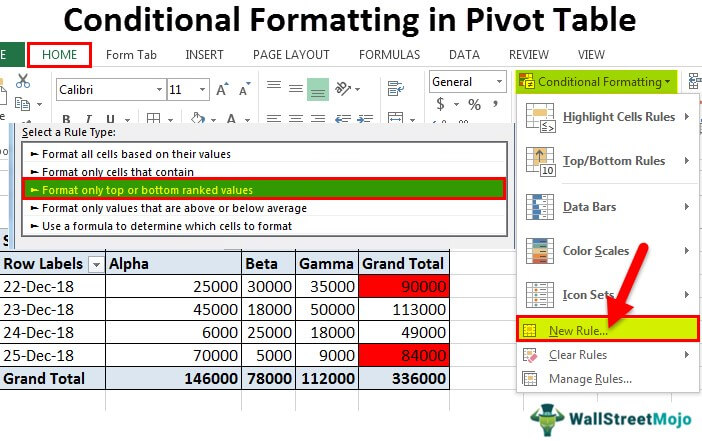
How to Apply Conditional Formatting in Pivot Table? (with ...
Conditional Formatting of Pivot Tables - Excel TV Conditional Formatting of Pivot Tables. Xtreme Pivot Tables. Current Progress. Current Progress. Current Progress 0% Not ... Change SUM Views in Label Areas. Indent Rows in Compact Layouts. Change Layout of a Report Filter. ... New Excel 2013 Pivot Table Features. Cosmetic Changes. Recommended Pivot Tables. Distinct Count. Timeline Slicer.

Working with Pivot Tables | Excel library | Syncfusion
Overwrite pivot table conditional format based on row label As far as I know, using the one rule in the Conditional formatting, we can only format the cells with one color if the condition is true and if the same condition is false, the formatting of the cell will be blank and if both conditions are true, the formatting of cell depends on the highest ranking/priority of the rules in Conditional formatting.
Pivot Table Conditional Formatting with VBA - Peltier Tech
Excel Conditional Formatting in Pivot Table - EDUCBA Click on any cell in the pivot table > Go to the HOME tab > Click on Conditional Formatting option under Styles option > Click on Manage Rules option. It will open a Rules Manager dialog box. Click on the Edit Rule tab, as shown in the below screenshot. It will open the Editing Rule formatting window. Refer to the below screenshot.
Pivot Table shows row labels instead of field name
Design the layout and format of a PivotTable - Microsoft Support To change the format of the PivotTable, you can apply a predefined style, banded rows, and conditional formatting. Windows Web Mac Changing the layout form of a PivotTable Change a PivotTable to compact, outline, or tabular form Change the way item labels are displayed in a layout form Change the field arrangement in a PivotTable

Add Pivot Table Conditional Formatting and Fix Problems
Pivot table conditional format based on row value | Chandoo.org Excel ... In the picture below you can see I have grouped some values together to form the row categories - I would like to tell excel to fill the cells with the data a different color where the row is "600-650" and a different color again for the row value "550-600" and so on for all the row categories shown.

microsoft excel - In a pivot table, how to apply conditional ...
Format Pivot Table Labels Based on Date Range Select all the dates in the Row Labels that you want to format. On the Ribbon, click the Home tab, and then in the Styles group, click Conditional Formatting. In the list of conditional formatting options, click Highlight Cells Rules, and then click A Date Occurring.
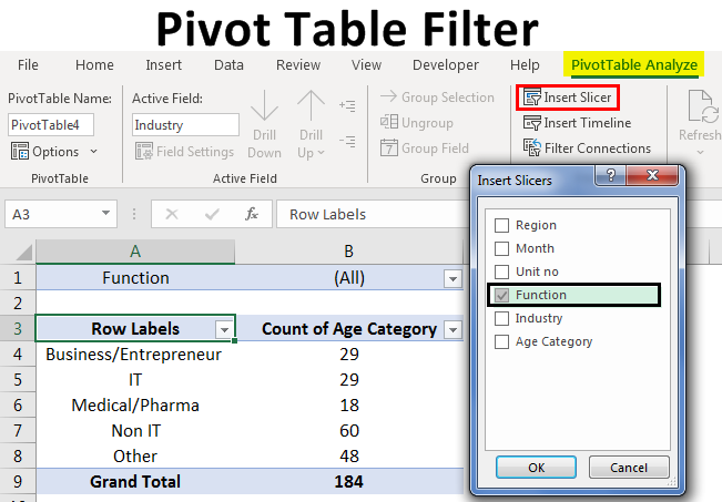
Pivot Table Filter | How to Filter Data in Pivot Table with ...
Using column label as formatting condition in excel pivot table I have pivot table in excel with sample data as attached. I now want to apply conditional formatting as red background where - data is between 10 to 25 AND - year is 2011 and 2012. =AND(C1="2011",OR(C2>10,C2<25)) how do i make cells example c2,c3,d2 red based on condition of year. Without Year condition it is working fine.
Applying Conditional Formatting to a Pivot Table in Excel
Formatting Pivot Table Row Labels by Level | MrExcel Message Board hover your cursor over the top line of one of the SubTotals of the Level that you want to format until you get a downward pointing, then left click - that should highlight all the cells at that level right click while hovering over one of the selected cells to format it OR hit Ctrl+F1
Conditional Formatting in Pivot Table (Example) | How To Apply?
Conditional Format Pivot Table Row | Chandoo.org Excel Forums - Become ... Select the entire row, and when you apply the conditional format, make the column reference absolute. So, say we want the entire row 2 to be formatted if cell in col B = 5. formula would be: =$B2=5

Learn How to Apply Conditional Formatting in a Pivot Table ...
Pivot Table Grouping, Ungrouping And Conditional Formatting 25 Oct 2022 — Conditional formatting is used to define rules to format data values in the table. It helps us to identify the important data easily in a large ...
Pivot Table Tips | Exceljet
Excel conditional formatting error - Microsoft Community Hub
Format Pivot Table Labels Based on Date Range | Excel Pivot ...

Pivot Table Grouping, Ungrouping And Conditional Formatting

Pivot Table Conditional Formatting - Microsoft Community Hub

How to apply conditional formatting to Pivot Tables
How to Apply Conditional Formatting to Pivot Tables - Excel ...

How to Apply Conditional Formatting in Pivot Table? (with ...

microsoft excel - In a pivot table, how to apply conditional ...

How to use Conditional Formatting in the Pivot table ...
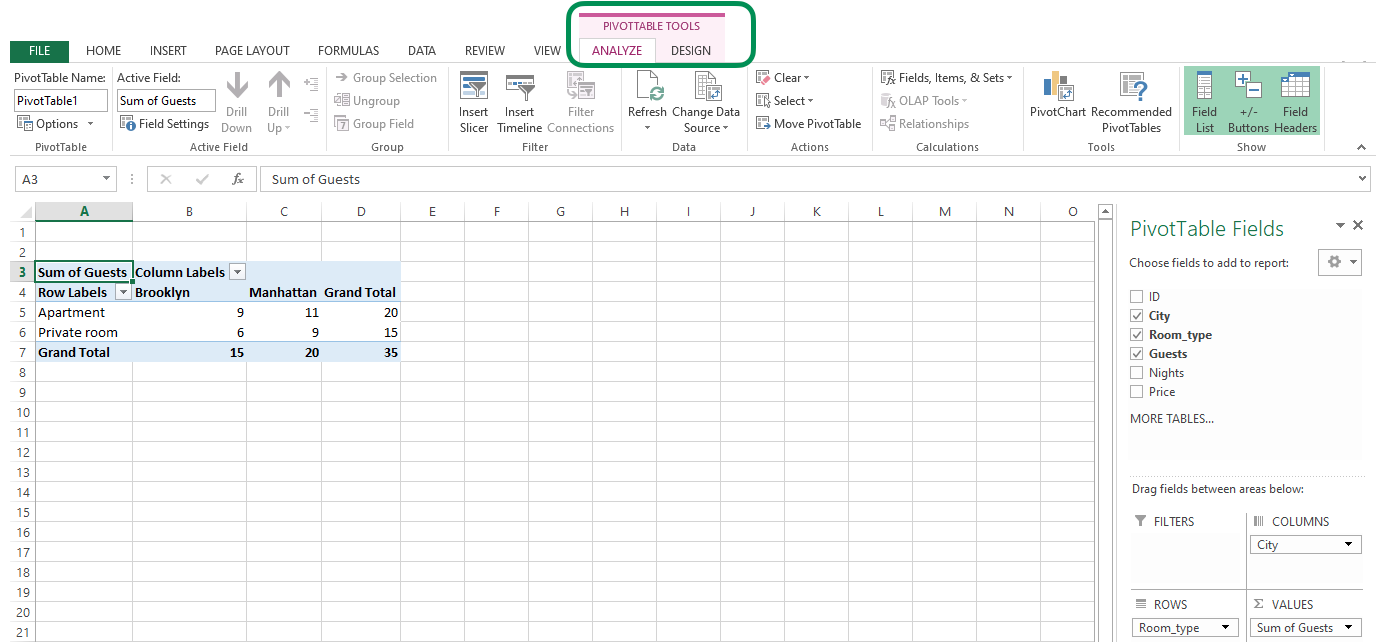
The Pivot table tools ribbon in Excel

Pivot Table Grouping, Ungrouping And Conditional Formatting
How to Apply Conditional Formatting to Rows Based on Cell ...

Conditional Formatting in Pivot Table (Example) | How To Apply?
How To Remove (blank) Values in Your Excel Pivot Table - MPUG

Pivot Table Conditional Formatting

vba - Pivot Table with Conditional Formatting: Where did my ...
How to Apply Conditional Formatting in Pivot Table? (with ...

Color-scale formatting dependent on each individual row in ...
Conditional Formatting for Pivot Table

How to Apply Conditional Formatting in Pivot Table? (with ...

Pivot Table Grouping, Ungrouping And Conditional Formatting

Using column label as formatting condition in excel pivot ...

Re-Apply Pivot Table Conditional Formatting - yoursumbuddy
Post a Comment for "39 excel pivot table conditional formatting row labels"