44 excel charts axis labels

Excel tutorial: How to customize axis labels Instead you'll need to open up the Select Data window. Here you'll see the horizontal axis labels listed on the right. Click the edit button to access the label range. It's not obvious, but you can type arbitrary labels separated with commas in this field. So I can just enter A through F. When I click OK, the chart is updated. Change axis labels in a chart in Office - support.microsoft.com In charts, axis labels are shown below the horizontal (also known as category) axis, next to the vertical (also known as value) axis, and, in a 3-D chart, next to the depth axis. The chart uses text from your source data for axis labels. To change the label, you can change the text in the source data.

Excel Chart: Horizontal Axis Labels won't update I created the data set in Excel 2016, selected the data and inserted a line chart. I sent one line to the secondary axis. The X axis still shows the correct labels. I sent the other line to the secondary axis and brought the first line back to the primary axis. The X axis labels are still correct. In short, I cannot reproduce the problem.

Excel charts axis labels

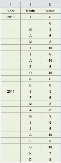
Excel charts: Labels on X-axis start at the wrong value If this does not work, you can also select the x-axis in the following way; assuming you are able to adjust the y-axis as mentioned in your comment. Select the y-axis -> right click -> Format Axis.... Inside Format Axis you need to select Axis Options and select Horizontal (Value) Axis: Share. edited yesterday. answered 2 days ago. How to add axis label to chart in Excel? - ExtendOffice You can insert the horizontal axis label by clicking Primary Horizontal Axis Title under the Axis Title drop down, then click Title Below Axis, and a text box will appear at the bottom of the chart, then you can edit and input your title as following screenshots shown. 4. Two-Level Axis Labels (Microsoft Excel) Excel automatically recognizes that you have two rows being used for the X-axis labels, and formats the chart correctly. (See Figure 1.) Since the X-axis labels appear beneath the chart data, the order of the label rows is reversed—exactly as mentioned at the first of this tip. Figure 1. Two-level axis labels are created automatically by Excel.

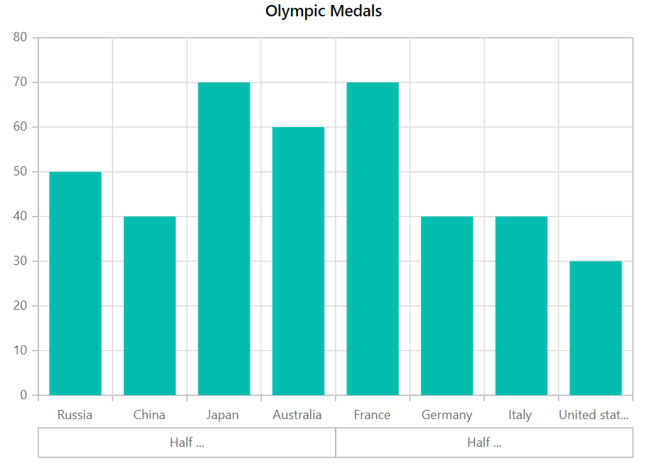
Excel charts axis labels. Change the display of chart axes - support.microsoft.com charts typically have two axes that are used to measure and categorize data: a vertical axis (also known as value axis or y axis), and a horizontal axis (also known as category axis or x axis). 3-d column, 3-d cone, or 3-d pyramid charts have a third axis, the depth axis (also known as series axis or z axis), so that data can be plotted along the … How do I add X-axis labels in Excel? - Yoforia.com Adding an Axis Title. Click the chart. From the Layout command tab, in the Labels group, click Axis Titles. To create a title for your x-axis, select Primary Horizontal Axis Title. Click the title location you desire. In the Axis Title text box, type a name for the axis. (Optional) To reposition your axis title, How to group (two-level) axis labels in a chart in Excel? Select the source data, and then click the Insert Column Chart (or Column) > Column on the Insert tab. Now the new created column chart has a two-level X axis, and in the X axis date labels are grouped by fruits. See below screen shot: Group (two-level) axis labels with Pivot Chart in Excel How to wrap X axis labels in a chart in Excel? - ExtendOffice And you can do as follows: 1. Double click a label cell, and put the cursor at the place where you will break the label. 2. Add a hard return or carriages with pressing the Alt + Enter keys simultaneously. 3. Add hard returns to other label cells which you want the labels wrapped in the chart axis.

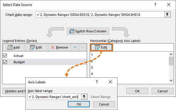
Excel charts: add title, customize chart axis, legend and data labels Click anywhere within your Excel chart, then click the Chart Elements button and check the Axis Titles box. If you want to display the title only for one axis, either horizontal or vertical, click the arrow next to Axis Titles and clear one of the boxes: Click the axis title box on the chart, and type the text. How to Add Axis Labels in Excel Charts - Step-by-Step (2022) First off, you have to click the chart and click the plus (+) icon on the upper-right side. Then, check the tickbox for 'Axis Titles'. If you would only like to add a title/label for one axis (horizontal or vertical), click the right arrow beside 'Axis Titles' and select which axis you would like to add a title/label. Editing the Axis Titles Add or remove data labels in a chart - support.microsoft.com In the upper right corner, next to the chart, click Add Chart Element > Data Labels. To change the location, click the arrow, and choose an option. If you want to show your data label inside a text bubble shape, click Data Callout. To make data labels easier to read, you can move them inside the data points or even outside of the chart. Change axis labels in a chart - support.microsoft.com Right-click the category labels you want to change, and click Select Data. In the Horizontal (Category) Axis Labels box, click Edit. In the Axis label range box, enter the labels you want to use, separated by commas. For example, type Quarter 1,Quarter 2,Quarter 3,Quarter 4. Change the format of text and numbers in labels

How to Add Axis Labels to a Chart in Excel Step 3: Select Axis Titles from the Chart Elements window. Once you have opened the Chart Elements window, you will see a number of items you can select to add to your chart. Check the Axis Titles option on the Chart Elements window and Axis Titles will appear on your chart. You can click on the arrow next to the Axis Titles option for some ... How to add Axis Labels (X & Y) in Excel & Google Sheets Adding Axis Labels Double Click on your Axis Select Charts & Axis Titles 3. Click on the Axis Title you want to Change (Horizontal or Vertical Axis) 4. Type in your Title Name Axis Labels Provide Clarity Once you change the title for both axes, the user will now better understand the graph. How to Label Axes in Excel: 6 Steps (with Pictures) - wikiHow Open your Excel document. Double-click an Excel document that contains a graph. If you haven't yet created the document, open Excel and click Blank workbook, then create your graph before continuing. 2. Select the graph. Click your graph to select it. 3. Click +. It's to the right of the top-right corner of the graph. How to Insert Axis Labels In An Excel Chart | Excelchat We will go to Chart Design and select Add Chart Element Figure 6 - Insert axis labels in Excel In the drop-down menu, we will click on Axis Titles, and subsequently, select Primary vertical Figure 7 - Edit vertical axis labels in Excel Now, we can enter the name we want for the primary vertical axis label.

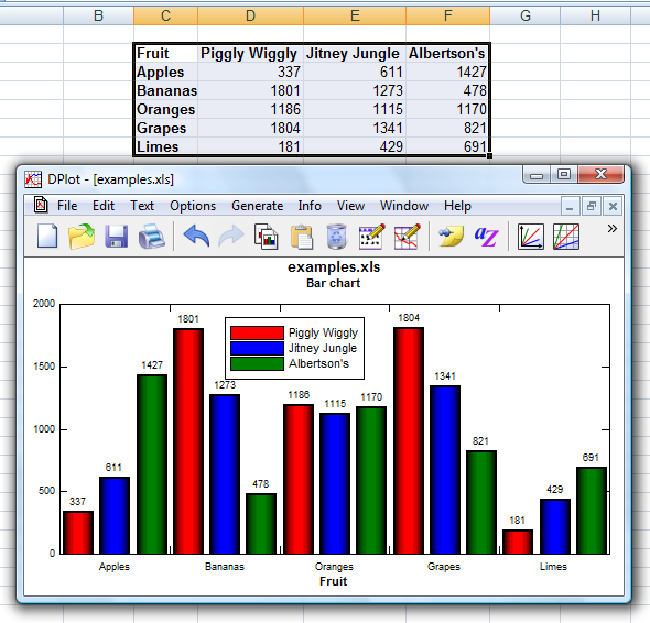
DPlot Windows software for Excel users to create presentation quality graphs

How To Add Axis Labels In Excel - BSUPERIOR Click on the chart area. Go to the Design tab from the ribbon. Click on the Add Chart Element option from the Chart Layout group. Select the Axis Titles from the menu. Select the Primary Vertical to add labels to the vertical axis, and Select the Primary Horizontal to add labels to the horizontal axis.

How to format the chart axis labels in Excel 2010 - YouTube

How to format axis labels individually in Excel - SpreadsheetWeb Double-clicking opens the right panel where you can format your axis. Open the Axis Options section if it isn't active. You can find the number formatting selection under Number section. Select Custom item in the Category list. Type your code into the Format Code box and click Add button. Examples of formatting axis labels individually

34 How To Label Chart Axis In Excel - Label Ideas 2020

How to rotate axis labels in chart in Excel? - ExtendOffice If you are using Microsoft Excel 2013, you can rotate the axis labels with following steps: 1. Go to the chart and right click its axis labels you will rotate, and select the Format Axis from the context menu. 2.

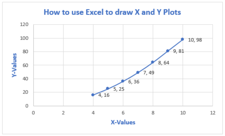
How To Plot X Vs Y Data Points In Excel | Excelchat

How to Add Axis Labels to a Chart in Excel | CustomGuide Select the set of gridlines you want to show. Add Data Labels Use data labels to label the values of individual chart elements. Select the chart. Click the Chart Elements button. Click the Data Labels check box. In the Chart Elements menu, click the Data Labels list arrow to change the position of the data labels. Display a Data Table

How To Rotate Axis Labels In Excel Chart - Best Picture Of Chart Anyimage.Org

Chart Axis - Use Text Instead of Numbers - Excel & Google Sheets Change Labels. While clicking the new series, select the + Sign in the top right of the graph. Select Data Labels. Click on Arrow and click Left. 4. Double click on each Y Axis line type = in the formula bar and select the cell to reference. 5. Click on the Series and Change the Fill and outline to No Fill. 6.

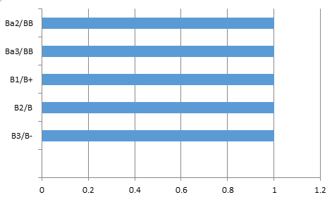
Bar charts with long category labels; Issue #428 November 27 2018 | Think Outside The Slide

How to change chart axis labels' font color and size in Excel? Right click the axis you will change labels when they are greater or less than a given value, and select the Format Axis from right-clicking menu. 2. Do one of below processes based on your Microsoft Excel version:

34 How To Label Chart Axis In Excel - Label Ideas 2020

Chart.Axes method (Excel) | Microsoft Docs This example adds an axis label to the category axis on Chart1. VB. With Charts ("Chart1").Axes (xlCategory) .HasTitle = True .AxisTitle.Text = "July Sales" End With. This example turns off major gridlines for the category axis on Chart1. VB.

Excel Chart X And Y Axis Labels - Chart Walls

Custom Axis Labels and Gridlines in an Excel Chart Select the horizontal dummy series and add data labels. In Excel 2007-2010, go to the Chart Tools > Layout tab > Data Labels > More Data Label Options. In Excel 2013, click the "+" icon to the top right of the chart, click the right arrow next to Data Labels, and choose More Options…. Then in either case, choose the Label Contains option ...

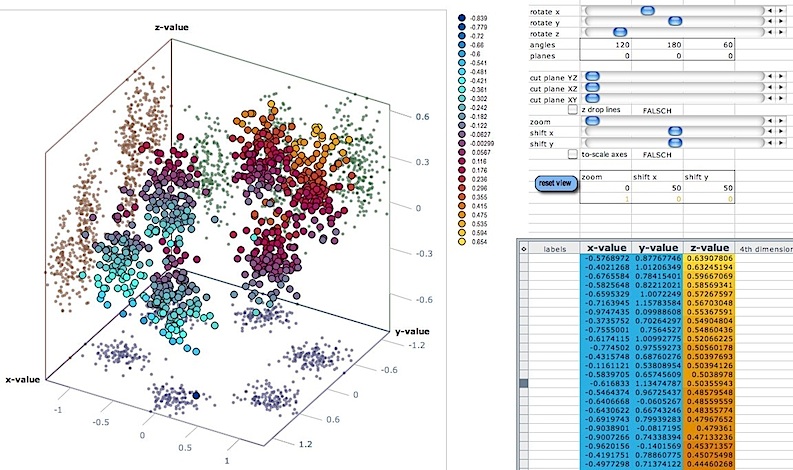
3d scatter plot for MS Excel

Format Chart Axis in Excel - Axis Options Formatting a Chart Axis in Excel includes many options like Maximum / Minimum Bounds, Major / Minor units, Display units, Tick Marks, Labels, Numerical Format of the axis values, Axis value/text direction, and more. However, there are a lot more formatting options for the chart axis, in this blog, we will be working with the axis options and ...

Dynamic Excel Dashboard: Dynamic Excel Charts using Drop Down List

How to Use Cell Values for Excel Chart Labels Select the chart, choose the "Chart Elements" option, click the "Data Labels" arrow, and then "More Options." Uncheck the "Value" box and check the "Value From Cells" box. Select cells C2:C6 to use for the data label range and then click the "OK" button. The values from these cells are now used for the chart data labels.

Axis Labels in Blazor Chart component - Syncfusion

Edit titles or data labels in a chart - support.microsoft.com On a chart, click the chart or axis title that you want to link to a corresponding worksheet cell. On the worksheet, click in the formula bar, and then type an equal sign (=). Select the worksheet cell that contains the data or text that you want to display in your chart. You can also type the reference to the worksheet cell in the formula bar.

Create Regular Excel Charts from PivotTables • My Online Training Hub

Two-Level Axis Labels (Microsoft Excel) Excel automatically recognizes that you have two rows being used for the X-axis labels, and formats the chart correctly. (See Figure 1.) Since the X-axis labels appear beneath the chart data, the order of the label rows is reversed—exactly as mentioned at the first of this tip. Figure 1. Two-level axis labels are created automatically by Excel.

30 Excel Chart Axis Label - 1000+ Labels Ideas

How to add axis label to chart in Excel? - ExtendOffice You can insert the horizontal axis label by clicking Primary Horizontal Axis Title under the Axis Title drop down, then click Title Below Axis, and a text box will appear at the bottom of the chart, then you can edit and input your title as following screenshots shown. 4.